Introduction

l0learn is a fast toolkit for L0-regularized learning. L0 regularization selects the best subset of features and can outperform commonly used feature selection methods (e.g., L1 and MCP) under many sparse learning regimes. The toolkit can (approximately) solve the following three problems

\begin{equation} \min_{\beta_0, \beta} \sum_{i=1}^{n} \ell(y_i, \beta_0+ \langle x_i, \beta \rangle) + \lambda ||\beta||_0 \quad \quad (L0) \end{equation}

\begin{equation} \min_{\beta_0, \beta} \sum_{i=1}^{n} \ell(y_i, \beta_0+ \langle x_i, \beta \rangle) + \lambda ||\beta||_0 + \gamma||\beta||_1 \quad (L0L1) \end{equation}

\begin{equation} \min_{\beta_0, \beta} \sum_{i=1}^{n} \ell(y_i, \beta_0+ \langle x_i, \beta \rangle) + \lambda ||\beta||_0 + \gamma||\beta||_2^2 \quad (L0L2) \end{equation}

where \(\ell\) is the loss function, \(\beta_0\) is the intercept, \(\beta\) is the vector of coefficients, and \(||\beta||_0\) denotes the L0 norm of \(\beta\), i.e., the number of non-zeros in \(\beta\). We support both regression and classification using either one of the following loss functions:

• Squared error loss

• Logistic loss (logistic regression)

• Squared hinge loss (smoothed version of SVM).

The parameter \(\lambda\) controls the strength of the L0 regularization (larger \(\lambda\) leads to less non-zeros). The parameter \(\gamma\) controls the strength of the shrinkage component (which is the L1 norm in case of L0L1 or squared L2 norm in case of L0L2); adding a shrinkage term to L0 can be very effective in avoiding overfitting and typically leads to better predictive models. The fitting is done over a grid of \(\lambda\) and \(\gamma\) values to generate a regularization path.

The algorithms provided in l0learn` are based on cyclic coordinate descent and local combinatorial search. Many computational tricks and heuristics are used to speed up the algorithms and improve the solution quality. These heuristics include warm starts, active set convergence, correlation screening, greedy cycling order, and efficient methods for updating the residuals through exploiting sparsity and problem dimensions. Moreover, we employed a new computationally efficient method for dynamically selecting the regularization parameter \(\lambda\) in the path. For more details on the algorithms used, please refer to our paper Fast Best Subset Selection: Coordinate Descent and Local Combinatorial Optimization Algorithms.

The toolkit is implemented in C++ along with an easy-to-use Python interface. In this vignette, we provide a tutorial on using the Python interface. Particularly, we will demonstrate how use L0Learn’s main functions for fitting models, cross-validation, and visualization.

Installation

L0Learn can be installed directly from pip by executing:

pip install l0learn

If you face installation issues, please refer to the Installation Troubleshooting Wiki. If the issue is not resolved, you can submit an issue on L0Learn’s Github Repo.

Tutorial

To demonstrate how l0learn works, we will first generate a synthetic dataset and then proceed to fitting L0-regularized models. The synthetic dataset (y,X) will be generated from a sparse linear model as follows:

• X is a 500x1000 design matrix with iid standard normal entries

• B is a 1000x1 vector with the first 10 entries set to 1 and the rest are zeros.

• e is a 500x1 vector with iid standard normal entries

• y is a 500x1 response vector such that y = XB + e

This dataset can be generated in python as follows:

import numpy as np
np.random.seed(4) # fix the seed to get a reproducible result
n, p, k = 500, 1000, 10
X = np.random.normal(size=(n, p))
B = np.zeros(p)
B[:k] = 1
e = np.random.normal(size=(n,))/2
y = X@B + e

More expressive and complete functions for generating datasets can be found are available in l0learn.models. The available functions are:

• l0learn.models.gen_synthetic()

• l0learn.models.gen_synthetic_high_corr()

• l0learn.models.gen_synthetic_logistic()

We will use l0learn to estimate B from the data (y,X). First we load L0Learn:

import l0learn

We will start by fitting a simple L0 model and then proceed to the case of L0L2 and L0L1.

Fitting L0 Regression Models

To fit a path of solutions for the L0-regularized model with at most 20 non-zeros using coordinate descent (CD), we use the l0learn.fit function as follows:

fit_model = l0learn.fit(X, y, penalty="L0", max_support_size=20)

This will generate solutions for a sequence of \(\lambda\) values (chosen automatically by the algorithm). To view the sequence of \(\lambda\) along with the associated support sizes (i.e., the number of non-zeros), we use the built-in rich display from ipython Rich Display for iPython Notebooks. When running this tutorial in a more standard python environment, use the function l0learn.models.FitModel.characteristics to display the sequence of solutions.

fit_model
# fit_model.characteristics()

	l0	support_size	intercept	converged
0	0.079546	0	-0.156704	True
1	0.078750	1	-0.147182	True
2	0.065862	2	-0.161024	True
3	0.050464	3	-0.002500	True
4	0.044517	5	-0.041058	True
5	0.041672	7	-0.058013	True
6	0.039705	8	-0.061685	True
7	0.032715	10	0.002157	True
8	0.000212	11	-0.000857	True
9	0.000187	12	-0.002161	True
10	0.000178	13	-0.001199	True
11	0.000159	15	-0.007959	True
12	0.000141	16	-0.009603	True
13	0.000133	18	-0.015697	True
14	0.000132	21	-0.012732	True

To extract the estimated B for particular values of \(\lambda\) and \(\gamma\), we use the function l0learn.models.FitModel.coeff. For example, the solution at \(\lambda = 0.032715\) (which corresponds to a support size of 10 + plus an intercept term) can be extracted using:

fit_model.coeff(lambda_0=0.032715, gamma=0)

<1001x1 sparse matrix of type '<class 'numpy.float64'>'
        with 11 stored elements in Compressed Sparse Column format>

The output is a sparse matrix of type scipy.sparse.csc_matrix. Depending on the include_intercept parameter of l0learn.models.FitModel.coeff, The first element in the vector is the intercept and the rest are the B coefficients. Aside from the intercept, the only non-zeros in the above solution are coordinates 0, 1, 2, 3, …, 9, which are the non-zero coordinates in the true support (used to generated the data). Thus, this solution successfully recovers the true support. Note that on some BLAS implementations, the lambda value we used above (i.e., 0.032715) might be slightly different due to the limitations of numerical precision. Moreover, all the solutions in the regularization path can be extracted at once by calling l0learn.models.FitModel.coeff without specifying a lambda_0 or gamma value.

The sequence of \(\lambda\) generated by L0Learn is stored in the object fit_model. Specifically, fit_model.lambda_0 is a list, where each element of the list is a sequence of \(\lambda\) values corresponding to a single value of \(\gamma\). When using an L0 penalty , which has only one value of \(\gamma\) (i.e., 0), we can access the sequence of \(\lambda\) values using fit.lambda_0[0]. Thus, \(\lambda=0.032715\) we used previously can be accessed using fit_model.lambda_0[0][7] (since it is the 8th value in the output of :code:fit.characteristics()). The previous solution can also be extracted using fit_model.coeff(lambda_0=0.032, gamma=0).

print(f"fit_model.lambda_0[0][7] = {fit_model.lambda_0[0][7]}")
fit_model.coeff(lambda_0=0.032715, gamma=0).toarray()

fit_model.lambda_0[0][7] = 0.03271533058913737

array([[0.00215713],
       [1.02014176],
       [0.97338278],
       ...,
       [0.        ],
       [0.        ],
       [0.        ]])

We can make predictions using a specific solution in the grid using the function fit_model.predict(newx, lambda, gamma) where newx is a testing sample (vector or matrix). For example, to predict the response for the samples in the data matrix X using the solution with \(\lambda=0.0058037\), we call the prediction function as follows:

with np.printoptions(threshold=10):
    print(fit_model.predict(x=X, lambda_0=0.032715, gamma=0))

[[-2.68272239]
 [-3.667317  ]
 [-1.77309853]
 ...
 [ 2.25545111]
 [-0.77364234]
 [-2.15002055]]

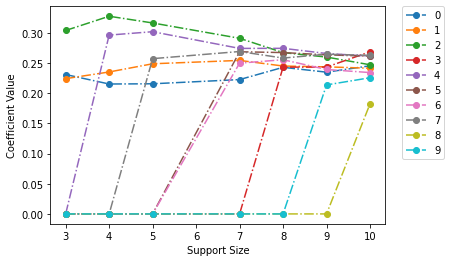
We can also visualize the regularization path by plotting the coefficients of the estimated B versus the support size (i.e., the number of non-zeros) using the l0learn.models.FitModel.plot() method as follows:

ax = fit_model.plot(include_legend=True)

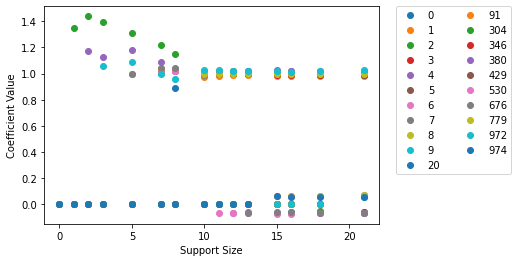
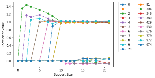
The legend of the plot presents the variables in the order they entered the regularization path. For example, variable 7 is the first variable to enter the path, and variable 6 is the second to enter. Thus, roughly speaking, we can view the first \(k\) variables in the legend as the best subset of size \(k\). To show the lines connecting the points in the plot, we can set the parameter :code:show_lines=True in the plot function, i.e., call :code:fit.plot(fit, gamma=0, show_lines=True). Moreover, we note that the plot function returns a matplotlib.axes._subplots.AxesSubplot object, which can be further customized using the matplotlib package. In addition, both the l0learn.models.FitModel.plot() and l0learn.models.CVFitModel.cv_plot() accept :code:**kwargs parameter to allow for customization of the plotting behavior.

fit_model.plot(show_lines=True)

<AxesSubplot:xlabel='Support Size', ylabel='Coefficient Value'>

Fitting L0L2 and L0L1 Regression Models

We have demonstrated the simple case of using an L0 penalty. We can also fit more elaborate models that combine L0 regularization with shrinkage-inducing penalties like the L1 norm or squared L2 norm. Adding shrinkage helps in avoiding overfitting and typically improves the predictive performance of the models. Next, we will discuss how to fit a model using the L0L2 penalty for a two-dimensional grid of :math:\lambda and :math:\gamma values. Recall that by default, l0learn automatically selects the :math:\lambda sequence, so we only need to specify the :math:\gamma sequence. Suppose we want to fit an L0L2 model with a maximum of 20 non-zeros and a sequence of 5 :math:\gamma values ranging between 0.0001 and 10. We can do so by calling l0learn.fit with :code:penalty="L0L2", :code:num_gamma=5, :code:gamma_min=0.0001, and :code:gamma_max=10 as follows:

fit_model_2 = l0learn.fit(X, y, penalty="L0L2", num_gamma = 5, gamma_min = 0.0001, gamma_max = 10, max_support_size=20)

l0learn will generate a grid of 5 :math:\gamma values equi-spaced on the logarithmic scale between 0.0001 and 10. Similar to the case for L0, we can display a summary of the regularization path using the l0learn.models.FitModel.characteristics function as follows:

fit_model_2 # Using ipython Rich Display
# fit_model_2.characteristics()  # For non Rich Display

	l0	support_size	intercept	converged	l2
0	0.003788	0	-0.156704	True	10.0000
1	0.003750	1	-0.156250	True	10.0000
2	0.002911	2	-0.148003	True	10.0000
3	0.002654	3	-0.148650	True	10.0000
4	0.002597	3	-0.148650	True	10.0000
...	...	...	...	...	...
128	0.000216	10	0.002130	True	0.0001
129	0.000173	13	-0.003684	True	0.0001
130	0.000167	13	-0.003685	True	0.0001
131	0.000134	18	-0.015724	True	0.0001
132	0.000130	21	-0.012762	True	0.0001

133 rows × 5 columns

The sequence of \(\gamma\) values can be accessed using fit_model_2.gamma. To extract a solution we use the l0learn.models.FitModel.coeff method. For example, extracting the solution at \(\lambda=0.0016\) and \(\gamma=10\) can be done using:

fit_model_2.coeff(lambda_0=0.0016, gamma=10)

<1001x1 sparse matrix of type '<class 'numpy.float64'>'
        with 11 stored elements in Compressed Sparse Column format>

Similarly, we can predict the response at this pair of \(\lambda\) and \(\gamma\) for the matrix X using

with np.printoptions(threshold=10):
    print(fit_model_2.predict(x=X, lambda_0=0.0016, gamma=10))

[[-0.31499242]
 [-0.3474209 ]
 [-0.23997924]
 ...
 [-0.06707991]
 [-0.18562493]
 [-0.25608131]]

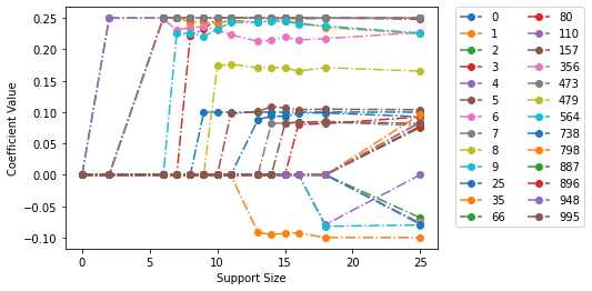
The regularization path can also be plotted at a specific \(\gamma\) using fit_model_2.plot(gamma=10). Here we can see the influence of ratio of \(\gamma\) and \(\lambda\). Since \(\gamma\) is so large (\(10\)) maintaining sparisity, then \(\lambda\) can be quite small \(0.0016\) which this results in a very stable estimate of the magnitude of the coeffs.

fit_model_2.plot(gamma=10, show_lines=True)

/Users/tnonet/Documents/GitHub/L0Learn/python/l0learn/models.py:438: UserWarning: Duplicate solution seen at support size 3. Plotting only first solution
  warnings.warn(f"Duplicate solution seen at support size {support_size}. Plotting only first solution")
/Users/tnonet/Documents/GitHub/L0Learn/python/l0learn/models.py:438: UserWarning: Duplicate solution seen at support size 10. Plotting only first solution
  warnings.warn(f"Duplicate solution seen at support size {support_size}. Plotting only first solution")
/Users/tnonet/Documents/GitHub/L0Learn/python/l0learn/models.py:438: UserWarning: Duplicate solution seen at support size 11. Plotting only first solution
  warnings.warn(f"Duplicate solution seen at support size {support_size}. Plotting only first solution")
/Users/tnonet/Documents/GitHub/L0Learn/python/l0learn/models.py:438: UserWarning: Duplicate solution seen at support size 12. Plotting only first solution
  warnings.warn(f"Duplicate solution seen at support size {support_size}. Plotting only first solution")

<AxesSubplot:xlabel='Support Size', ylabel='Coefficient Value'>

Finally, we note that fitting an L0L1 model can be done by just changing the penalty to “L0L1” in the above (in this case gamma_max will be ignored since it is automatically selected by the toolkit; see the reference manual for more details.)

Higher-quality Solutions using Local Search

By default, l0learn uses coordinate descent (CD) to fit models. Since the objective function is non-convex, the choice of the optimization algorithm can have a significant effect on the solution quality (different algorithms can lead to solutions with very different objective values). A more elaborate algorithm based on combinatorial search can be used by setting the parameter algorithm="CDPSI" in the call to l0learn.fit. CDPSI typically leads to higher-quality solutions compared to CD, especially when the features are highly correlated. CDPSI is slower than CD, however, for typical applications it terminates in the order of seconds.

Cross-validation

We will demonstrate how to use K-fold cross-validation (CV) to select the optimal values of the tuning parameters \(\lambda\) and \(\gamma\). To perform CV, we use the l0learn.cvfit function, which takes the same parameters as l0learn.fit, in addition to the number of folds using the num_folds parameter and a seed value using the seed parameter (this is used when randomly shuffling the data before performing CV).

For example, to perform 5-fold CV using the L0L2 penalty (over a range of 5 gamma values between 0.0001 and 0.1) with a maximum of 50 non-zeros, we run:

cv_fit_result = l0learn.cvfit(X, y, num_folds=5, seed=1, penalty="L0L2", num_gamma=5, gamma_min=0.0001, gamma_max=0.1, max_support_size=50)

Note that the object returned during cross validation is l0learn.models.CVFitModel which subclasses l0learn.models.FitModel and thus has the same methods and underlinying structure. The cross-validation errors can be accessed using the cv_means attribute of a CVFitModel: cv_fit_result.cv_means is a list where the ith element, cv_fit_result.cv_means[i], stores the cross-validation errors for the ith value of gamma cv_fit_result.gamma[i]). To find the minimum cross-validation error for every gamma, we apply the :code:np.argmin function for every element in the list :cv_fit_result.cv_means, as follows:

gamma_mins = [(i, np.argmin(cv_mean), np.min(cv_mean)) for i, cv_mean in enumerate(cv_fit_result.cv_means)]
gamma_mins

[(0, 8, 0.5313128699361661),
 (1, 8, 0.2669789604993652),
 (2, 8, 0.2558807301729078),
 (3, 20, 0.25555788170828786),
 (4, 19, 0.2555564968851251)]

The above output indicates that the 5th value of gamma achieves the lowest CV error (=0.255). We can plot the CV errors against the support size for the 5th value of gamma, i.e., gamma = cv_fit_result.gamma[4], using:

cv_fit_result.cv_plot(gamma = cv_fit_result.gamma[4])
cv_fit_result.cv_sds

<AxesSubplot:xlabel='Support Size', ylabel='Cross-Validation Error'>

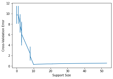
The above plot is produced using the matplotlib package and returns a matplotlib.axes._subplots.AxesSubplot which can be further customized by the user. We can also note that we have error bars in the cross validation error which is stored in cv_sds attribute and can be accessed with cv_fit_result.cv_sds. To extract the optimal \(\lambda\) (i.e., the one with minimum CV error) in this plot, we execute the following:

optimal_gamma_index, optimal_lambda_index, min_error = min(gamma_mins, key = lambda t: t[2])
print(optimal_gamma_index, optimal_lambda_index, min_error)
print("Optimal lambda = ", fit_model_2.lambda_0[optimal_gamma_index][optimal_lambda_index])

4 19 0.2555564968851251
Optimal lambda =  0.0016080760437896327

To print the solution corresponding to the optimal gamma/lambda pair:

cv_fit_result.coeff(lambda_0=fit_model_2.lambda_0[optimal_gamma_index][optimal_lambda_index],
                    gamma=fit_model_2.gamma[optimal_gamma_index])

<1001x1 sparse matrix of type '<class 'numpy.float64'>'
        with 11 stored elements in Compressed Sparse Column format>

The optimal solution (above) selected by cross-validation correctly recovers the support of the true vector of coefficients used to generate the model.

beta_vector = cv_fit_result.coeff(lambda_0=fit_model_2.lambda_0[optimal_gamma_index][optimal_lambda_index],
                    gamma=fit_model_2.gamma[optimal_gamma_index],
                    include_intercept=False).toarray()

with np.printoptions(threshold=30, edgeitems=15):
    print(np.hstack([beta_vector, B.reshape(-1, 1)]))

[[1.01994648 1.        ]
 [0.97317979 1.        ]
 [0.99813347 1.        ]
 [0.99669481 1.        ]
 [1.01128182 1.        ]
 [1.00190748 1.        ]
 [1.01272103 1.        ]
 [0.99204841 1.        ]
 [0.99607406 1.        ]
 [1.0266543  1.        ]
 [0.         0.        ]
 [0.         0.        ]
 [0.         0.        ]
 [0.         0.        ]
 [0.         0.        ]
 ...
 [0.         0.        ]
 [0.         0.        ]
 [0.         0.        ]
 [0.         0.        ]
 [0.         0.        ]
 [0.         0.        ]
 [0.         0.        ]
 [0.         0.        ]
 [0.         0.        ]
 [0.         0.        ]
 [0.         0.        ]
 [0.         0.        ]
 [0.         0.        ]
 [0.         0.        ]
 [0.         0.        ]]

Fitting Classification Models

All the commands and plots we have seen in the case of regression extend to classification. We currently support logistic regression (using the parameter loss="Logistic") and a smoothed version of SVM (using the parameter loss="SquaredHinge"). To give some examples, we first generate a synthetic classification dataset (similar to the one we generated in the case of regression):

import numpy as np
np.random.seed(4) # fix the seed to get a reproducible result
n, p, k = 500, 1000, 10
X = np.random.normal(size=(n, p))
B = np.zeros(p)
B[:k] = 1
e = np.random.normal(size=(n,))/2
y = np.sign(X@B + e)

More expressive and complete functions for generating datasets can be found are available in l0learn.models. The available functions are:

• l0learn.models.gen_synthetic()

• l0learn.models.gen_synthetic_high_corr()

• l0learn.models.gen_synthetic_logistic()

An L0-regularized logistic regression model can be fit by specificying loss = "Logistic" as follows:

fit_model_3 = l0learn.fit(X,y,loss="Logistic", max_support_size=20)
fit_model_3

	l0	support_size	intercept	converged	l2
0	25.225336	1	-0.036989	True	1.000000e-07
1	19.432053	2	-0.043199	True	1.000000e-07
2	18.928603	2	-0.043230	True	1.000000e-07
3	15.142882	2	-0.043245	True	1.000000e-07
4	12.114306	9	0.004044	True	1.000000e-07
5	7.411211	10	0.188422	False	1.000000e-07
6	7.188875	10	0.219990	False	1.000000e-07
7	5.751100	10	0.234899	False	1.000000e-07
8	4.600880	10	0.242631	False	1.000000e-07
9	3.680704	10	0.243655	True	1.000000e-07
10	2.944563	10	0.243993	True	1.000000e-07
11	2.355651	10	0.244295	True	1.000000e-07
12	1.884520	10	0.244520	True	1.000000e-07
13	1.507616	10	0.244716	True	1.000000e-07
14	1.206093	10	0.244886	True	1.000000e-07
15	0.964874	10	0.245011	True	1.000000e-07
16	0.771900	10	0.245133	True	1.000000e-07
17	0.617520	12	0.178144	False	1.000000e-07
18	0.598994	12	0.196406	False	1.000000e-07
19	0.479195	12	0.208883	False	1.000000e-07
20	0.383356	15	0.192033	False	1.000000e-07
21	0.371856	15	0.221470	False	1.000000e-07
22	0.297484	15	0.246182	False	1.000000e-07
23	0.237988	16	-0.110626	False	1.000000e-07
24	0.230848	16	-0.118558	False	1.000000e-07
25	0.184678	16	-0.124533	False	1.000000e-07
26	0.147743	21	-0.211002	False	1.000000e-07

The output above indicates that \(\gamma=10^{-7}\) by default we use a small ridge regularization (with \(\gamma=10^{-7}\)) to ensure the existence of a unique solution. To extract the coefficients of the solution with \(\lambda = 8.69435\) we use the following code. Notice that we can ignore the specification of gamma as there is only one gamma used in L0 Logistic regression:

np.where(fit_model_3.coeff(lambda_0=7.411211).toarray() > 0)[0]

The above indicates that the 10 non-zeros in the estimated model match those we used in generating the data (i.e, L0 regularization correctly recovered the true support). We can also make predictions at the latter \(\lambda\) using:

with np.printoptions(threshold=10):
   print(fit_model_3.predict(X, lambda_0=7.411211))

[[1.69583037e-04]
 [4.92440655e-06]
 [3.92195535e-03]
 ...
 [9.99161941e-01]
 [1.69035746e-01]
 [9.99171256e-04]]

Each row in the above is the probability that the corresponding sample belongs to class \(1\). Other models (i.e., L0L2 and L0L1) can be similarly fit by specifying loss = "Logistic".

Finally, we note that L0Learn also supports a smoothed version of SVM by using squared hinge loss loss = "SquaredHinge". The only difference from logistic regression is that the predict function returns \(\beta_0 + \langle x, \beta \rangle\) (where \(x\) is the testing sample), instead of returning probabilities. The latter predictions can be assigned to the appropriate classes by using a thresholding function (e.g., the sign function).

Advanced Options

Sparse Matrix Support

Starting in version 2.0.0, L0Learn supports sparse matrices of type scipy.sparse.csc_matrix. If your sparse matrix uses a different storage format, please convert it to csc_matrix before using it in l0learn. l0learn keeps the matrix sparse internally and thus is highly efficient if the matrix is sufficiently sparse. The API for sparse matrices is the same as that of dense matrices, so all the demonstrations in this vignette also apply for sparse matrices. For example, we can fit an L0-regularized model on a sparse matrix as follows:

from scipy.sparse import random
from scipy.stats import norm


X_sparse = random(n, p, density=0.01, format='csc', data_rvs=norm().rvs)
y_sparse = (X_sparse@B + e)

fit_model_sparse = l0learn.fit(X_sparse, y_sparse, penalty="L0", max_support_size=20)

fit_model_sparse.characteristics()

	l0	support_size	intercept	converged
0	0.031892	0	0.009325	True
1	0.031573	1	0.004882	True
2	0.020606	2	-0.002187	True
3	0.014442	3	-0.004111	True
4	0.013932	4	-0.002556	True
5	0.010854	5	0.002987	True
6	0.009286	6	0.002048	True
7	0.009191	7	-0.001371	True
8	0.008771	8	-0.000533	True
9	0.008151	9	0.000064	True
10	0.006480	11	0.001587	True
11	0.006364	12	-0.003636	True
12	0.005760	13	-0.003866	True
13	0.005560	15	-0.004211	True
14	0.005264	17	0.001497	True
15	0.004637	18	-0.000797	True
16	0.004515	19	-0.002634	True
17	0.004113	22	0.001419	True

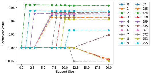
Selection on Subset of Variables

In certain applications, it is desirable to always include some of the variables in the model and perform variable selection on others. l0learn supports this option through the exclude_first_k parameter. Specifically, setting exclude_first_k = K (where K is a non-negative integer) instructs l0learn to exclude the first K variables in the data matrix X from the L0-norm penalty (those K variables will still be penalized using the L2 or L1 norm penalties.). For example, below we fit an L0 model and exclude the first 3 variables from selection by setting excludeFirstK = 3:

fit_model_k = l0learn.fit(X, y, penalty="L0", max_support_size=10, exclude_first_k=3)
fit_model_k.characteristics()

	l0	support_size	intercept	converged
0	0.050464	3	-0.017599	True
1	0.044333	4	-0.021333	True
2	0.032770	5	-0.027624	True
3	0.029367	7	-0.029115	True
4	0.024710	8	-0.021199	True
5	0.021393	9	0.010249	True
6	0.014785	10	0.016812	True

Plotting the regularization path:

fit_model_k.plot(show_lines=True)

<AxesSubplot:xlabel='Support Size', ylabel='Coefficient Value'>

We can see in the plot above that first 3 variables, (0, 1, 2) are included in all the solutions of the path

Coefficient Bounds

Starting in version 2.0.0, l0learn supports bounds for CD algorithms for all losses and penalties. (We plan to support bound constraints for the CDPSI algorithm in the future). By default, l0learn does not apply bounds, i.e., it assumes \(-\infty <= \beta_i <= \infty\) for all i. Users can supply the same bounds for all coefficients by setting the parameters lows and highs to scalar values (these should satisfy: lows <= 0, lows != highs, and highs >= 0). To use different bounds for the coefficients, lows and highs can be both set to vectors of length p (where the i-th entry corresponds to the bound on coefficient i).

All of the following examples are valid.

l0learn.fit(X, y, penalty="L0", lows=-0.5)
l0learn.fit(X, y, penalty="L0", highs=0.5)
l0learn.fit(X, y, penalty="L0", lows=-0.5, highs=0.5)

max_value = 0.25
highs_array = max_value*np.ones(p)
highs_array[0] = 0.1
fit_model_bounds = l0learn.fit(X, y, penalty="L0", lows=-0.1, highs=highs_array, max_support_size=20)

We can see the coefficients are subject to the bounds.

fit_model_bounds.plot(show_lines=True)

print(f"maximum value of coefficients = {np.max(fit_model_bounds.coeffs[0])} <= {max_value}")
print(f"maximum value of first coefficient = {np.max(fit_model_bounds.coeffs[0][0, :])} <= 0.1")
print(f"minimum value of coefficient = {np.min(fit_model_bounds.coeffs[0])} >= -0.1")

/Users/tnonet/Documents/GitHub/L0Learn/python/l0learn/models.py:438: UserWarning: Duplicate solution seen at support size 0. Plotting only first solution
  warnings.warn(f"Duplicate solution seen at support size {support_size}. Plotting only first solution")
/Users/tnonet/Documents/GitHub/L0Learn/python/l0learn/models.py:438: UserWarning: Duplicate solution seen at support size 6. Plotting only first solution
  warnings.warn(f"Duplicate solution seen at support size {support_size}. Plotting only first solution")
/Users/tnonet/Documents/GitHub/L0Learn/python/l0learn/models.py:438: UserWarning: Duplicate solution seen at support size 8. Plotting only first solution
  warnings.warn(f"Duplicate solution seen at support size {support_size}. Plotting only first solution")

maximum value of coefficients = 0.25 <= 0.25
maximum value of first coefficient = 0.1 <= 0.1
minimum value of coefficient = -0.1 >= -0.1

User-specified Lambda Grids

By default, l0learn selects the sequence of lambda values in an efficient manner to avoid wasted computation (since close \(\lambda\) values can typically lead to the same solution). Advanced users of the toolkit can change this default behavior and supply their own sequence of \(\lambda\) values. This can be done supplying the \(\lambda\) values through the parameter lambda_grid. When lambda_grid is supplied, we require num_gamma and num_lambda to be None to ensure the is no ambiguity in the solution path requested.

Specifically, the value assigned to lambda_grid should be a list of lists/arrays of decreasing positive values (floats). The length of lambda_grid (the number of lists stored) specifies the number of gamma parameters that will fill between gamma_min, and gamma_max. In the case of L0 penalty, lambda_grid must be a list of length 1. In case of L0L2/L0L1 lambda_grid can have any number of sub-lists stored. The ith element in lambda_grid should be a strictly decreasing sequence of positive lambda values which are used by the algorithm for the ith value of gamma. For example, to fit an L0 model with the sequence of user-specified lambda values: 1, 1e-1, 1e-2, 1e-3, 1e-4, we run the following:

user_lambda_grid = [[1, 1e-1, 1e-2, 1e-3, 1e-4]]
fit_grid = l0learn.fit(X, y, penalty="L0", lambda_grid=user_lambda_grid, max_support_size=1000, num_lambda=None, num_gamma=None)

To verify the results we print the fit object:

fit_grid
# Use fit_grid.characteristics() for those without rich dispalys

	l0	support_size	intercept	converged
0	1.0000	0	-0.016000	True
1	0.1000	0	-0.016000	True
2	0.0100	10	0.016811	True
3	0.0010	62	0.018729	True
4	0.0001	267	0.051675	True

Note that the \(\lambda\) values above are the desired values. For L0L2 and L0L1 penalties, the same can be done where the lambda_grid parameter.

user_lambda_grid_L2 = [[1, 1e-1, 1e-2, 1e-3, 1e-4],
                       [10, 2, 1, 0.01, 0.002, 0.001, 1e-5],
                       [1e-4, 1e-5]]

# user_lambda_grid_L2[[i]] must be a sequence of positive decreasing reals.
fit_grid_L2 = l0learn.fit(X, y, penalty="L0L2", lambda_grid=user_lambda_grid_L2, max_support_size=1000, num_lambda=None, num_gamma=None)

fit_grid_L2
# Use fit_grid_L2.characteristics() for those without rich dispalys

	l0	support_size	intercept	converged	l2
0	1.00000	0	-0.016000	True	10.000000
1	0.10000	0	-0.016000	True	10.000000
2	0.01000	0	-0.016000	True	10.000000
3	0.00100	9	-0.014394	True	10.000000
4	0.00010	134	-0.012180	True	10.000000
5	10.00000	0	-0.016000	True	0.031623
6	2.00000	0	-0.016000	True	0.031623
7	1.00000	0	-0.016000	True	0.031623
8	0.01000	10	0.015045	True	0.031623
9	0.00200	28	0.001483	True	0.031623
10	0.00100	58	0.002821	True	0.031623
11	0.00001	582	0.021913	True	0.031623
12	0.00010	311	0.048700	True	0.000100
13	0.00001	411	0.047991	False	0.000100

More Details

For more details please inspect the doc strings of:

• l0learn.models.CVFitModel

• l0learn.models.FitModel

• l0learn.fit

• l0learn.cvfit

References

Hussein Hazimeh and Rahul Mazumder. Fast Best Subset Selection: Coordinate Descent and Local Combinatorial Optimization Algorithms. Operations Research (2020).

Antoine Dedieu, Hussein Hazimeh, and Rahul Mazumder. Learning Sparse Classifiers: Continuous and Mixed Integer Optimization Perspectives. JMLR (to appear).